Ex-2: Thermal simulation of a heat sink
The Rhino and Grasshopper files used in this example are available for download
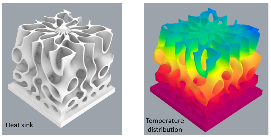
This example demonstrates how to simulate heat transfer of a heat sink as shown in the picture below. This geometry is generated in nTop.
The key steps involved in setting up the simulation are explained here.
New users are advised to checkout the getting started page to understand the basics of using the plugin.
Geometry and material setup
Create a geometry object on the canvas. Set the geometry to the heat sink, and let’s name this geometry as “heat sink” as shown in (a)
Create an Intact component and connect the heat sink block’s output to the component as shown in (b)
Create an Intact thermal material block. Right click on the block and choose Aluminum 6061 as the material (c).

Applying thermal loads
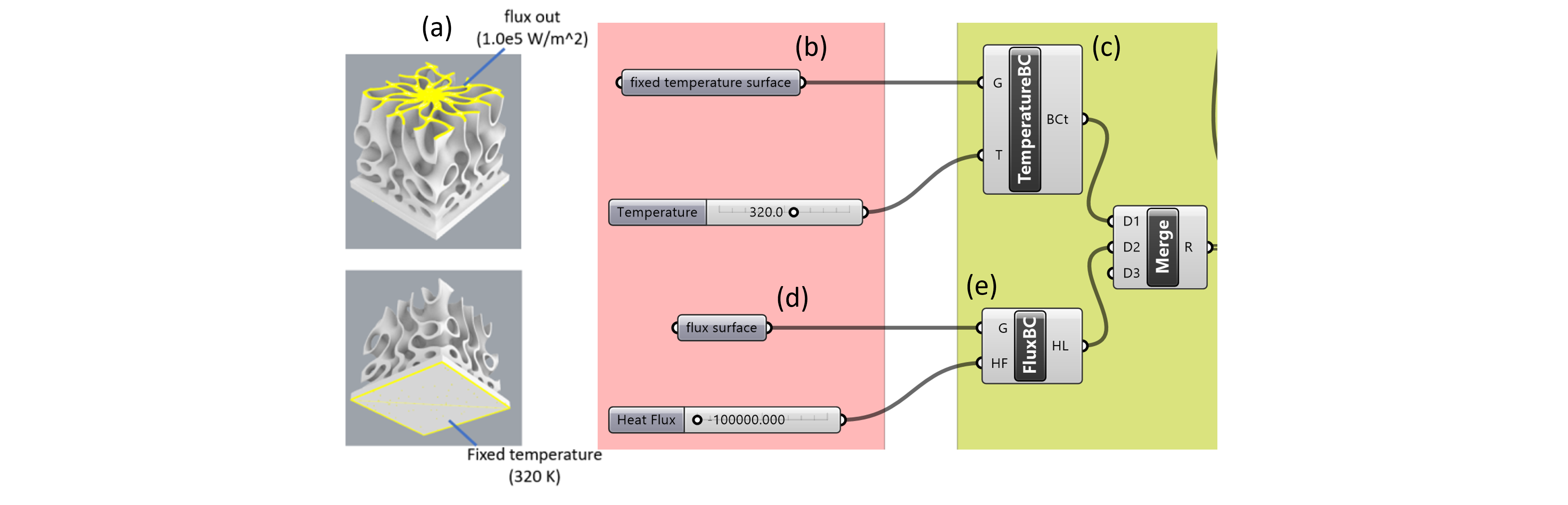
The load and restraint surfaces are shown in (a) below
Create a geometry object and set it to the bottom surface. Let’s name this geometry as “fixed temperature surface” as shown in (b)
Create a Temperature boundary condition block as connect the fixed temperature surface block’s output to the component as shown in (c)
Create a geometry object and set it to the top surface. Let’s name this geometry as “flux surface” as shown in (d)
Create a “flux boundary condition” block and connect the flux surface and the flux magnitude of -1.0E5 W/m2, as shown in (e)
Merge the temperature and flux boundary condition blocks as shown in (f)
Setup solver
Create a solver settings block as shown in (a)
Set the target resolution of 100K
Select the linear solver type (direct)
Select the basis order ( basis order = 1 for linear elements)
Set up the solver block as shown in (b)
Connect the solver settings (SS)
Connect the heat sink (C)
Connect the merged boundary condition block (BCt)
Hit solve to compute the solution

Setup visualization block
Create a visualization block (b) and connect the solver output to the visualization block
Optionally, users can connect the visualization settings block for customizing the views
Right click on the visualize block and choose the simulation output for display (e.g. temperature or heat flux).

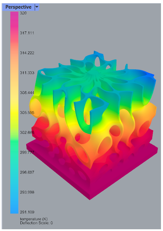
The temperature distribution of the bonded assembly is displayed below, which shows that the max-min temperature is approximately 320K and 292K, respectively.