Overview
Introduction to the API
This document provides a comprehensive guide to using our Python API for Intact.Simulation. The API allows users to define geometries, material properties, components, assemblies, and boundary conditions. Users can specify units, create simulation scenarios, execute the simulation, and query the results. The simulations can be run with different solver types and the results can be written to a file for visualization. The document also provides Python code examples and snippets for each step of the simulation process.
Key features and capabilities
Physics support
Linear elasticity
Modal
Thermal
Linear buckling
Thermoelasticity
Geometry Support
Brep: Surface mesh
VDB volume
Level set topology optimization
Getting Started
A simple example of running a structural simulation. Any geometry files used in these examples are available in the
examples/folder.Import Intact Module
from pyintact import *
Create Geometry
beam_geometry = MeshModel("beam.stl")
beam_geometry.instance_id = "simple_cantilever"
beam_geometry.refine(0.02) # refine stl for smoother visualization
Create Material (Properties are in MKS unit system)
material = IsotropicMaterialDescriptor() # steel
material.density = 7800.0 # kg/m^3
material.poisson_ratio = 0.3
material.youngs_modulus = 2.1e11 # Pa
Create Restraints and Loads
# Create a fixed boundary condition at one end of the beam
fixed_boundary = FixedBoundaryDescriptor()
fixed_boundary.boundary = MeshModel("restraint.stl")

# Create a pressure load at the free end of the beam
pressure_load = PressureForceDescriptor()
pressure_load.units = UnitSystem.MeterKilogramSecond
pressure_load.magnitude = 1000  # Applying pressure in Pascals
pressure_load.boundary = MeshModel("load.stl")
Setup simulation and solve
# Setup the simulation scenario descriptor
scenario = LinearElasticScenarioDescriptor()
scenario.materials = {"Steel": material}
scenario.metadata.resolution = 10000
scenario.metadata.units = UnitSystem.MeterKilogramSecond
scenario.boundary_conditions = [fixed_boundary, pressure_load]

# Associate the material with the model
component = MaterialDomain(beam_geometry, "Steel", scenario)
assembly = [component]

# Initialize and run the simulator
simulator = StressSimulator(assembly, scenario)
simulator.solve()
Query result and create output file to visualize
# Query results for stress distribution
results = QueryResult(assembly)
stress_query = FieldQuery(Field.VonMisesStress)
simulator.sample(stress_query, results)

# Write results to a file (unit system is saved as a metadata in the vtu file)
results.writeVTK("cantilever_beam_results.vtu", UnitSystem.MeterKilogramSecond)
How To
Creating Simulation Input
Units
The default Unit System is MKS or MeterKilogramSecond. We
allow the following customizations:
Specify custom unit for geometry through the
Scenariounit (default MKS)Specify custom unit for loads (default MKS)
Specify custom unit for materials (default MKS)
Unit System Keywords |
Mass |
Force |
Stress |
Length |
Temperature |
Energy |
|---|---|---|---|---|---|---|
MeterKilogramSecond |
kg |
N |
Pa |
m |
K |
J |
CentimeterGramSecond |
g |
dyne |
dyne/cm² |
cm |
K |
dyne·cm |
MillimeterMegagramSecond |
Mg |
N |
MPa |
mm |
K |
mJ |
FootPoundSecond |
slug |
lbf |
lbf/ft² |
ft |
Ra |
lbf·ft |
InchPoundSecond |
lbf s²/in (slinch) |
lbf |
psi |
in |
Ra |
lbf·in |
Geometry
Geometry is specified through a Model object
MeshModelfrom surface mesh can be defined in two ways.filenameto define mesh from a file (STL, PLY)instance_ida unique name
mesh_geometry = MeshModel(filename="beam.stl")
mesh_geometry.instance_id = "beam"
Constructing mesh face-by-face
# define an empty mesh
mesh_geometry = MeshModel()
mesh_geometry.instance_id = "fixed_boundary"

# add vertices to the mesh and get the vertex id as output
v0 = mesh_geometry.addVertex([0.0, 0.0, 0.0])
v1 = mesh_geometry.addVertex([1.0, 0.0, 0.0])
v2 = mesh_geometry.addVertex([0.0, 1.0, 0.0])

# add faces defined by the vertex id
mesh_geometry.addFacet(v0, v1, v2)
Mesh refinement (usually used for finer interpolation of results during visualization). Uses
MeshModel.refinewithrefinement_levelas an input which is the largest allowed triangle edge as a ratio of the bounding box diagonal.# mesh geometry created above is further refined mesh_geometry.refine(refinement_level=0.02)
VDB Model
Using a
.vdbfilevdb_geometry= VDBModel("box.vdb")
In memory using a
VDBobjectimport pyopenvdb as vdb # create a vdb double grid object cube = vdb.DoubleGrid() cube.fill(min=(100, 100, 100), max=(199, 199, 199), value=1.0) # create an Intact Model from VDB object vdb_geometry = pyintact.VDBModel(cube) # create a tesselation of the vdb to get a MeshModel and its list of vertices for sampling mesh = vdb_geometry.tesselate() # mesh is a MeshModel() num_vertices = mesh.vertexCount() print(num_vertices)
Material Properties
Structural
IsotropicMaterialDescriptorto create an Isotropic material. (Unit isMeterKilogramSecond)densityis the material densityyoungs_modulusis the elastic moduluspoisson_ratiois the Poisson ratio
steel_structural = IsotropicMaterialDescriptor()

# Set the density to 7845 kg/m^3, modulus to 200 GPa and poison ratio to 0.29
steel_structural.density = 7845
steel_structural.youngs_modulus = 200e9
steel_structural.poisson_ratio = 0.29
OrthotropicMaterialDescriptorto create an Orthotropic material. Orthotropic materials are often used to represent composites and wood, where the material properties along one axis are significantly different from the properties along the other axes. (Unit isMeterKilogramSecond)densityis the material densityExis the elastic modulus in the material’s x-directionEyis the elastic modulus in the material’s y-directionEzis the elastic modulus in the material’s z-directionGxyis the shear modulus in the xy planeGxzis the shear modulus in the xz planeGyzis the shear modulus in the yz planevxyis the poisson ratio in the xy planevxzis the poisson ratio in the xx planevyzis the poisson ratio in the yz planetransformis the optional material transform to arbitrarily rotate the axes along which the material properties are defined. Specified as a list of 9 floating point numbers corresponding to a 3x3 matrix. Note the first 3 floating point numbers corresponds to the first row.
# Create an orthotropic material (Red Pine)
material = OrthotropicMaterialDescriptor()
material.density = 460.0             # kg/m³
material.Ex = 11.2e9                 # Pa
material.Ey = 492.8e6                # Pa
material.Ez = 985.6e6                # Pa
material.Gxy = 907.2e6               # Pa
material.Gxz = 1.08e9                # Pa
material.Gyz = 123.2e6               # Pa
material.vxy = 0.315
material.vxz = 0.347
material.vyz = 0.308
material.transform = [1.0, 0.0, 0.0,
                    0.0, 1.0, 0.0,
                    0.0, 0.0, 1.0] # optional in this case
Thermal
ThermalMaterialDescriptorto create a thermal material. (Default unit isMeterKilogramSecond)densityis the material densityconductivityis the conductivity of the materialspecific_heatis the specific heat of the material
thermal_material = ThermalMaterialDescriptor()

# Set the density, conductivity, and specific heat of the material
thermal_material.density = 2700.0 # kg/m^3
thermal_material.conductivity = 170  # W/(m·K)
thermal_material.specific_heat = 500  # J/(kg·K)

# Optionally set the coefficient of thermal expansion when using
# the thermal material in a thermo linear elasticity scenario.
thermal_material.expansion_coefficient = 23.0e-6
Component and Assembly
A Component is created as a
MaterialDomainand takes three inputsA
Modelobject (MeshModelorVDBModelspecifically)A material name
A
ScenarioDescriptorobject
bar1_structural = MaterialDomain(mesh_geometry, "Steel", structural_scenario)
bar2_structural = MaterialDomain(vdb_geometry, "Steel", structural_scenario)
Assembly is a
listof components that are bonded togetherstructural_assembly = [bar1_structural, bar2_structural]
Boundary Conditions
Restraints
Fixed Boundary A “Fixed Boundary” restraint fixes the selected geometry in all directions.
The fixed boundary only has one input:
the
boundarysurface to be fixed
fixed = FixedVectorDescriptor()

# Set the geometry "restraint.ply" to be fixed
fixed.boundary = MeshModel("restraint.ply")
Fixed Vector A “Fixed Vector” restraint allows for each direction to be optionally set to a specified displacement value, 0 being fixed and ‘None’ being un-restrained. Note that a structural problem must have all three directions restrained somewhere to be valid.
A fixed vector has five inputs:
the
boundarysurface to be fixedthe
x_valueto set the displacement for the x-axis direction (optional)the
y_valueto set the displacement for the y-axis direction (optional)the
z_valueto set the displacement for the z-axis direction (optional)the
unitsthat apply to the displacement values
fixed_vector = FixedVectorDescriptor()

# Set the geometry "restraint.stl" to be restrained
fixed_vector.boundary = MeshModel("restraint.stl")

# Set the displacements in each direction
fixed_vector.x_value = 0.2  # X-direction displacement of 0.2 ft
fixed_vector.y_value = None # un-restrained in the Y-direction at this surface
fixed_vector.z_value = 0.0  # fixed Z-direction
fixed_vector.units = UnitSystem.FootPoundSecond
Sliding Restraint A “Sliding Restraint” allows for motion tangential to a specified surface, but fixes motion normal to the specified surface.
A sliding restraint only has one input:
the
boundarysurface for the sliding restraint condition
sliding_boundary = SlidingBoundaryDescriptor()

# Set the geometry "restraint.stl" for the sliding restraint condition
sliding_boundary.boundary = MeshModel("restraint.stl")
Structural Loads (
TractionDescriptor)Vector Force
“Vector Force” load is a surface load applied to a face in a specified direction. An example of this load is pressing on the top of a book to push it across a table.
A vector load requires four inputs:
the
boundarysurfaces where the load is appliedthe
directionvector of the forcethe
unitsthat apply to the magnitudethe
magnitudeof the force.
load = VectorForceDescriptor()

# Set the geometry "load.stl" the vector load is applied to
load.boundary = MeshModel("load.stl")

# Set the vector load direction to be in the -Z direction with a magnitude of 100 lbf
load.direction = [0, 0, -1]
load.units = UnitSystem.InchPoundSecond
load.magnitude = 100 # lbf
Torque
“Torque” load is a surface load that applies a twisting force around an axis. The direction of the torque is determined using the right-hand rule: using your right hand, point your thumb in the direction of the axis. A positive torque value applies a torque acting in the direction the fingers of your right hand would wrap around the axis. The torque load is applied among the load faces with a distribution that varies linearly from zero at the axis.
A Torque load requires five inputs:
the
boundarysurfaces where the load is appliedthe
axisof rotation about which the torque actsoriginis the starting point of the axis of rotationthe
unitsthat apply to the magnitudemagnitudeof the torque.
torque_load = TorqueForceDescriptor()

# Set the geometry "load.stl" the torque load is applied to
torque_load.boundary = MeshModel("load.stl")

# Set the axis of the torque axis
torque_load.origin = (10, 1, 1)
torque_load.axis = [1, 0, 0] # Set the torque to be about the +X (right-hand rule)
torque_load.units = UnitSystem.MeterKilogramSecond
torque_load.magnitude = 10 # Set the torque magnitude to 10 N*m
Pressure
A “Pressure” load is a surface load specified in terms of force per unit area. Positive pressures ‘push’ into the surface, and negative pressures ‘pull’.
A Pressure Load requires three inputs:
the
boundarysurfaces where the load is appliedthe
unitsthat apply to the magnitudethe
magnitudeof the pressure.
pressure_load = PressureForceDescriptor()

# Set the geometry "load.stl" the pressure load is applied to
pressure_load.boundary = MeshModel("load.stl")

# Set the pressure magnitude to 10 Pa
pressure_load.units = UnitSystem.MeterKilogramSecond
pressure_load.magnitude = 10
Bearing Force
A “Bearing Force” is a surface load applied to a (typically) cylindrical face to approximate the effects of a shaft pressing against the side of a hole. The applied force gets converted to a varying pressure distribution on the portion of the face experiencing compressive pressure. The pressure distribution is computed automatically to achieve the specified overall bearing force.
A Bearing Force requires four inputs:
the
boundarysurfaces where the load is appliedthe
directionvector of the bearing forcethe
unitsthat apply to the magnitudethe
magnitudeof the force
bearing_load = BearingForceDescriptor()

# Set the geometry "load.stl" the bearing load is applied to
bearing_load.boundary = MeshModel("load.stl")

# Set the loading direction to be in the -Z
bearing_load.direction = [0, 0, -1]

# Set the magnitude of the load to 100 N
bearing_load.units = UnitSystem.MeterKilogramSecond
bearing_load.magnitude = 100
Hydrostatic Load
A “Hydrostatic” load is a spatially varying pressure on the surfaces submerged in a fluid due to the weight of that fluid. The pressure at any point depends on the height and density of the fluid, increasing from zero at the fluid surface to a maximum at the deepest point.
A Hydrostatic load requires four inputs:
the
boundarysurfaces where the load is appliedthe
heightof the fluid surfacethe
densityof the fluidthe
unitsthat apply to the fluid height and density
# Create a hydrostatic load on a face of the box
hydrostatic_load = HydrostaticForceDescriptor()

# Set the geometry "load.stl" the hydrostatic load is applied to
hydrostatic_load.boundary = MeshModel("load.stl")

# Set the fluid height to 78.0 cm with a fluid density of 1.00 g/cm^3
hydrostatic_load.units = UnitSystem.CentimeterGramSecond
hydrostatic_load.height = 78
hydrostatic_load.density = 1.0
Flexible Remote Load
A “Flexible Remote Load” allows specifying the force and moment at a remote location that is then applied to a surface. It can be used in a similar manner to NASTRAN’s RBE3 load or Abaqus coupling elements.
A Flexible Remote Load requires seven inputs:
the
boundarysurfaces where the load is appliedthe
directionvector of the remote forcethe
forceof the remote forcethe
axisof rotation about which the moment actsthe
momentmagnitude of the remote momentthe
remote_pointwhere the force and moment are appliedthe
unitsthat apply to the magnitude and moment
The
directionandaxisvectors should be unit vectors to describe the direction. They will be normalized if they are not unit vectors.load = FlexibleRemoteLoadDescriptor() # Set the geometry "load.stl" the load is applied to load.boundary = MeshModel("load.stl") # Set the loading direction to be in the -Y load.direction = [0, -1, 0] # Set the magnitude of the load to 100 N load.units = UnitSystem.MeterKilogramSecond load.magnitude = 100 # Set the moment axis in the X direction load.axis = [1, 0, 0] # Set the magnitude of the moment to 200 N-m load.moment = 200 # The remote load acts at the point (1, 1, 1) load.remote_point = [1, 1, 1]
Thermal Loads
Fixed Boundary (Fixed Temperature)
A “Fixed Boundary” load fixes the selected geometry to a specified temperature when the
valueis specified and non-zero.The fixed boundary has three inputs:
the
boundarysurface to be fixedthe
valueof the temperature to fix at the boundary surfacethe
unitsthat apply to the temperature (SI - K, English - Ra)
fixed = FixedBoundaryDescriptor()

# Set the geometry "fixed_temp.ply" to set a fixed temperaure of 320 K
fixed_boundary.boundary = MeshModel("fixed_temp.ply")
fixed_boundary.value = 320  # Kelvin

# Set the geometry "fixed_temp.ply" to set a fixed temperaure of 500 Rankine
fixed_boundary.boundary = MeshModel("fixed_temp.ply")
fixed_boundary.units = UnitSystem.InchPoundSecond
fixed_boundary.value = 500  # Rankine
Convection
A “Convection” load specifies the transfer of heat from a surrounding medium.
A thermal convection boundary condition requires three inputs:
the
boundarysurface(s) where the convection is applied.the heat transfer
coefficientthe
environment_temperatureof the surrounding mediumthe
units(default MKS)
# Create an instance of ConvectionDescriptor
convection = ConvectionDescriptor()
convection.units = UnitSystem.MeterKilogramSecond

# Set the geometry "face.ply" the convection is applied to
convection.boundary = MeshModel("face.ply")

# Set the heat transfer coefficient to 25 W/m^2K and environment temperature
convection.coefficient = 25  # W/m^2K
convection.environment_temperature = 300  # Kelvin
Surface Flux
Surface “Thermal or Heat Flux” specifies the heat flow per unit of surface area.
A surface thermal flux requires two inputs:
the
boundarysurface(s) where the flux is applied.the
magnitudeof the heat fluxthe
units(default MKS)
# Create an instance of ConstantFluxDescriptor
flux = ConstantFluxDescriptor()
flux.units = UnitSystem.MeterKilogramSecond

# Set the geometry "face.ply" the constant flux is applied to
flux.boundary = MeshModel("face.ply")

# Set the flux magnitude to 500 W/m^2
flux.magnitude = 500  # W/m^2
Body Loads/Internal Conditions
Body loads comprise forces that are distributed over a solid volume.
Linear Acceleration Load or Gravity
A linear acceleration load can be used to simulate the effect of gravity. The material in the body will tend to be pulled in the direction of the acceleration vector. A linear accleration body load is configured by specifying the direction of the acceleration and its magnitude.
The inputs to the body load are:
the
directionvector of the acceleration fieldthe
unitsthat apply to the magnitudethe
magnitudeof acceleration
# Example for a "gravity load"
body_load = BodyLoadDescriptor()

# Set the direction vector to be downward (-Z)
body_load.direction = [0, 0, -1]

# Set the magnitude to 9.80655 m/s^2
body_load.units = UnitSystem.MeterKilogramSecond
body_load.magnitude = 9.80665
Rotational Load
Rotational body loads simulate the effect of a body rotating around an axis. Two contributions are considered in a rotational body load: angular velocity and angular acceleration. The angular velocity term simulates the centrifugal effects that tend to throw a body’s material away from the axis of rotation. The angular acceleration term simulates the effect of a rotational acceleration field around the axis of rotation. A positive angular acceleration tends to drag the body’s material in the positive rotational direction according to the right-hand rule.
A rotational body load has 4 inputs:
originpoint for the axis of rotationvector defining the
axisof rotationangular_velocity(in radians/sec)angular_acceleration(in radians/sec²)
rotational_load = RotationalLoadDescriptor()

# Set the origin at the coordinate system origin
rotational_load.origin = (0, 0, 0)

# Set the axis of rotation about the y-axis
rotational_load.axis = [0, 1, 0]

# Set angular velocity to 10 rad/s and angular acceleration to 0.5 rad/s^2
rotational_load.angular_velocity = 10
rotational_load.angular_acceleration = 0.5
Thermal Loads
Constant Heat
A “Constant Heat” or body heat flux load applies uniform heat generation over a specified volume.
Constant heat flux has 2 inputs
the
instance_idof the components which are producing heat fluxthe
magnitudeof the body heat fluxthe
units(default MKS)
constant_heat = ConstantHeatDescriptor()
constant_heat.units = UnitSystem.MeterKilogramSecond

# Set the heat generation to -200,000 W/m^3 for a beam component
constant_heat.instance_id = "beam"
constant_heat.magnitude = -200000.0  # W/m^3
Simulation Scenario Setup and Solution
Scenario Setup using
ScenarioDescriptorLinear Elasticity scenario is created using
LinearElasticScenarioDescriptor. It takes the following inputs:boundary_conditions, a list of boundary conditionsinternal_conditions, a list of internal conditions (body loads)
Scenario Metadata,
metadata, a set of solver parameters to control the accuracy and speed of the simulation:resolutionis the target number of finite elements. An iterative process determines acell_sizethat achieves approximately the specified number of elements. You can directly specify thecell_sizeinstead ofresolution. Note that decreasingcell_sizecan quickly result in large numbers of finite elements and long solve times.resolutionis recommended for most cases.unitssets the unit of the scenario (geometry and results will be in this unit) for example, a geometry in ‘MKS’ that is 6 m long would be 6 mm long when set to ‘MMS’.basis_orderis the type of finite element used. The default is 1, which would be linear elements. 2 is for quadratic elements.solver_typeis the solver type used in the simulation with the following options:MKL_PardisoLDLT(default) is the direct solver and is typically faster for lower resolution (< 200K cells on 32 GB memory), but gets slower and consumes more memory at higher resolutionsAMGCL_amg_rigid_bodyis the iterative solver which is typically faster at high resolution.
scenario = LinearElasticScenarioDescriptor()
scenario.materials = {"Aluminum 6061-T6": material}
scenario.boundary_conditions = [fixed_boundary, vector_load, torque_load]
scenario.internal_conditions = [body_load]

scenario.metadata.resolution = 10000
scenario.metadata.units = UnitSystem.MeterKilogramSecond

# Optional settings
scenario.metadata.basis_order = 2 # 2 = quadratic elements
scenario.metadata.solver_override = Solver.AMGCL_amg_rigid_body # iterative solver
Similarly, Modal scenario is created using
ModalScenarioDescriptorwhich takesboundary_conditions, a list of boundary conditions, as input.The
metadatais the same as for the linear elastic scenario except there is necessary inputmodal_metadata.desired_eigenvaluesthat takes in an integer for the number of eigenvalues.
# Setup the modal simulation scenario
modal_scenario = ModalScenarioDescriptor()
modal_scenario.materials = {"Aluminum 6061-T6": material}
modal_scenario.boundary_conditions = [fixed_boundary]

modal_scenario.metadata.resolution = 10000
modal_scenario.modal_metadata.desired_eigenvalues = 10

# Optional settings
modal_scenario.metadata.basis_order = 2 # 2 = quadratic elements
modal_scenario.metadata.solver_override = Solver.AMGCL_amg_rigid_body  #iterative solver
Similarly, Linear Buckling scenario is created using
LinearBucklingScenarioDescriptorwhich takesboundary_conditions, a list of boundary conditions, as input. A linear buckling scenario first performs a linear elasticity simulation, and then solves a generalized eigenvalue problem to determine the critical load factors.The
metadatais the same as for the linear elastic scenario except there is necessary inputbuckling_metadata.desired_eigenvaluesthat takes in an integer for the number of eigenvalues.
# Setup the linear buckling simulation scenario
buckling_scenario = LinearBucklingScenarioDescriptor()
buckling_scenario.materials = {"Aluminum 6061-T6": material}
buckling_scenario.boundary_conditions = [fixed_boundary]

buckling_scenario.metadata.resolution = 10000
# Generally, the first critical load factor from a buckling analysis is most useful,
# a small number of additional buckling modes may be useful to examine.
buckling_scenario.buckling_metadata.desired_eigenvalues = 3

# Optional settings
buckling_scenario.metadata.basis_order = 2 # 2 = quadratic elements
# Use iterative solver for the linear elasticity simulation
buckling_scenario.metadata.solver_override = Solver.AMGCL_amg_rigid_body
Similarly, a Thermal scenario is created using
StaticThermalScenarioDescriptorwhich takes a list ofboundary_conditionsand a list ofinternal_conditionsas input. Note that thematerialmust be a thermal material for this scenario type.The
metadatais the same as for the linear elastic scenario with additional inputthermal_metadata.environment_temperaturewhich specifies the temperature of the environment.
# Setup the thermal simulation scenario
thermal_scenario = StaticThermalScenarioDescriptor()
thermal_scenario.materials = {"Aluminum 6061-T6": material}
thermal_scenario.boundary_conditions = [fixed_temp, convection]
thermal_scenario.internal_conditions = [constant_heat]
thermal_scenario.thermal_metadata.environment_temperature = 300.0

thermal_scenario.metadata.resolution = 10000

# Optional settings
thermal_scenario.metadata.basis_order = 2 # 2 = quadratic elements
thermal_scenario.metadata.solver_override = Solver.AMGCL_amg # iterative solver
A Thermoelasticity scenario is created by creating a thermal scenario, solving the thermal simulation, then creating a linear elasticity scenario, and solving it:
RESOLUTION = 10000
# Setup the thermal simulation scenario
thermal_scenario = StaticThermalScenarioDescriptor()
thermal_scenario.materials = {"Aluminum 6061-T6": material}
thermal_scenario.boundary_conditions = [fixed_temp, convection]
thermal_scenario.internal_conditions = [constant_heat]
thermal_scenario.thermal_metadata.environment_temperature = 300.0
thermal_scenario.metadata.resolution = RESOLUTION

# Solve the thermal scenario
thermal_simulator = StaticThermalSimulator(assembly, thermal_scenario)
thermal_simulator.solve()

# Setup the linear elastic simulation scenario
scenario = LinearElasticScenarioDescriptor()
scenario.materials = {"Aluminum 6061-T6": material}
scenario.boundary_conditions = [fixed_boundary, vector_load, torque_load]
scenario.internal_conditions = [body_load]

scenario.metadata.resolution = RESOLUTION

# Solve the thermo linear elastic scenario
simulator = StressSimulator(assembly, scenario, thermal_simulator)
simulator.solve()
Note
For best results, the thermal scenario resolution should be the same or less than the stress scenario resolution. Using the same resolution ensures that the thermal fields are defined every where the stress simulation will be performed.
Note
Ensure that the material used for the thermal scenario has an expansion coefficient defined, so the calculated thermal field can be used in the linear elasticity scenario to determine the thermally induced strain.
Finalize Simulation Setup and Execute
Stress Simulation is created using
StressSimulator. It takes the following inputs:An
assemblyor the list ofMaterialDomainsLinearElasticScenarioDescriptorthat describes the simulation scenario
# Initialize and run the linear elastic scenario
simulator = StressSimulator(assembly, scenario)
simulator.solve()
Modal Simulation is created using
ModalSimulator. It takes the following inputs:An
assemblyor the list ofMaterialDomainsModalScenarioDescriptorthat describes the simulation scenario
# Initialize and run the modal scenario
modal_simulator = ModalSimulator(assembly, modal_scenario)
modal_simulator.solve()
Linear Buckling Simulation is created using
LinearBucklingSimulator. It takes the following inputs:An
assemblyor the list ofMaterialDomainsLinearBucklingScenarioDescriptorthat describes the simulation scenario
# Initialize and run the linear buckling scenario
buckling_simulator = LinearBucklingSimulator(assembly, buckling_scenario)
buckling_simulator.solve()
Static Thermal Simulation is created using
StaticThermalSimulator. It takes the following inputs:An
assemblyor the list ofMaterialDomainsStaticThermalScenarioDescriptorthat describes the simulation scenario
# Initialize and run the static thermal scenario
thermal_simulator = StaticThermalSimulator(assembly, thermal_scenario)
thermal_simulator.solve()
Query and Result Output
Create a
QueryResultobject that specifies the domain to be sampled. It takes a singlecomponentor anassemblyas input.assembly = [component_1, component_2] results = QueryResult(component_1) # sample only the defined component results = QueryResult(assembly) # sample on the full assembly
Specify a query class and type that defines what quantity you are querying. The query classes and types available are as follows :
Global Query is for querying quantities defined for the entire domain or structure. The available
GlobalQueryTypes areCompliance,ReactionForce,TotalReactonForce,TotalReactionMoment,TotalAppliedForce, andTotalAppliedMomentfor linear elasticity simulations,Frequencyfor modal simulations,CriticalLoadFactorfor linear buckling simulations, andThermalCompliancefor static thermal simulations.TotalReactionForceis a tuple of dimension 3 containing the total reaction force[x-force, y-force, z-force]
ReactionForceis a tuple of dimension 3 for each restrained boundary, in the order the boundary conditions were added to theLinearElasticScenarioDescriptor.[x-force, y-force, z-force]
TotalReactionMomentis 3 tuples of dimension 3, representing the moments about the origin generated by reaction forces. Using [r1, r2, r3] to represent the vector from the origin to the reaction force, and using [Fx, Fy, Fz] to represent the reaction force, the moments are:[0, r2 * Fx, r3 * Fx] [r1 * Fy, 0, r3 * Fy] [r1 * Fz, r2 * Fz, 0]
TotalAppliedForceis a tuple of dimension 3, representing the total applied load.[Fx, Fy, Fz]
TotalAppliedMomentis 3 tuples of dimension 3, representing the moments about the origin generated by the applied loads. Using [r1, r2, r3] to represent the vector from the origin to the applied load, and using [Fx, Fy, Fz] to represent the applied load, the moments are:[0, r2 * Fx, r3 * Fx] [r1 * Fy, 0, r3 * Fy] [r1 * Fz, r2 * Fz, 0]
# GlobalQuery example
# Create a GlobalQuery to query the first mode
results = QueryResult(assembly)
frequency_query = GlobalQuery(GlobalQueryType.Frequency, DiscreteIndex(0))

# Sample the simulation for the specified query
freq_1 = simulator.sample(mode1_query, results)
print(freq_1.get(0,0)) # Print out the first mode in Hz

# Example use to get the first 10 modes
# Note, the simulator would need this:
# modal_scenario.modal_metadata.desired_eigenvalues = 10

for i in range(10):
    # Create the query for the current mode
    query = GlobalQuery(GlobalQueryType.Frequency, DiscreteIndex(i))

    # Sample the query using the simulator
    r = simulator.sample(query, results)

    # Append the value obtained from result.get(0, 0) to a list
    values.append(r.get(0, 0))
    print(values) # list of first 10 modes in Hz
Field Query is for querying field quantities defined at any point in the domain. The available field quantities depend on the physics type.
For Stress Simulation, the following
FieldTypeinputs are availableDisplacementtuple of dimension 3 for each point[x-displacement, y-displacement, z-displacement]
StrainandStressare each a tuple of dimension 6 for each point[stress_xx, stress_yy, stress_zz, stress_yz, stress_xz, stress_xy] [strain_xx, strain_yy, strain_zz, strain_yz, strain_xz, strain_xy]
TopologicalSensitivity,StrainEnergyDensity, andVonMisesStressare each a tuple of dimension 1 for each point
For Modal Simulation and Linear Buckling Simulation, the only
FieldTypeavailable isDisplacement, which corresponds to the mode shape information and requires an index for the specified mode.# Create a field query for the displacement/mode shape of mode 1 mode_num = 0 # first mode modal_field_query = FieldQuery(f=Field.Displacement, scheme=DiscreteIndex(mode_num))
For Thermal Simulation, the available
FieldTypes areTemperaturewhich is a tuple of dimension 1HeatFluxwhich is a tuple of dimension 3
Field Query Interface usage
# FieldQuery example
# Create a FieldQuery to query displacement
results = QueryResult(assembly)
displacement_query = FieldQuery(f=Field.Displacement)

# Create a FieldQuery with optional input to query the y-component
y_displacement_query = FieldQuery(f=Field.Displacement, component=1)

# FieldQuery with optional input to query the norm of displacement
displacement_magnitude_query = FieldQuery(f=Field.Displacement, norm=True)

# Sample the simulation with the given query to create a VectorArray
# * more info on VectorArrays are provided in the subsequent section *
displacement_VectorArray1 = simulator.sample(displacement_query, results)
displacement_VectorArray2 = simulator.sample(y_displacement_query, results)
displacement_VectorArray3 = simulator.sample(displacement_magnitude_query, results)

displacement1 = displacement_VectorArray1.get(i, j); # jth component of the displacement (0 = X, 1 = Y, or 2 = Z) at the ith sampling point
displacement2 = displacement_VectorArray2.get(1, 0); # y-displacement value at the second sampling point
displacement3 = displacement_VectorArray3.get(1, 0); # displacement magnitude at the second sampling point
Statistical queries allow querying for the maximum, minimum or mean of any field quantity. The following example queries for the maximum von Mises stress.
# Create a StatisticalQuery to query for the maximum von Mises stress
results = QueryResult(assembly)
max_von_mises_query = StatisticalQuery(f=Field.VonMisesStress, s=StatisticalQueryType.Maximum)

max_von_mises = simulator.sample(max_von_mises_query, results).get(0, 0)
Sample and Export Results
Sampling results in-memory
Methods to sample results of the simulation and store/print
VectorArrayresults from the queries created above.# Query results results = QueryResult(assembly) stress_query = FieldQuery(f=Field.Stress) # a field is needed to create a field query stress_VectorArray = simulator.sample(stress_query, results)
This sampling is stored in a
VectorArrayof sizen_tuplebydimension,n_tupleis the number of points sampled in the component/assembly and dimension depends on the query type. For example,FieldQuery(Field.Displacement)has a dimension of 3 for each displacement component, thusVectorArray.get(i, 2)would get the z-displacement of pointi.# Get the number of tuples (vectors) in the VectorArray (one per point results are sampled at) n_tuples = stress_VectorArray.n_tuples() # Get the dimension of each vector - in this case 6, one value for each stress component dimension = stress_VectorArray.dimension() stress_xx = stress_VectorArray.get(i, 0); # stress_xx at i-th sample point stress_yy = stress_VectorArray.get(i, 1); # stress_yy at i-th sample point stress_ij = stress_VectorArray.get(i, j); # jth stress component (0, 1, 2, 3, 4, or 5) of the ith tuple
Export results to a file: Once the query is created,
resultscan be used to write a.vtufile which contains all solution fields viaresults.writeVTKwhich has two inputs:file name
"*.vtu"UnitSystemis an attribute in the*.vtu( Note that this argument is just metadata in the*.vtufile. The result magnitudes are in the unit of the scenario regardless of the unit system specified. )
# Write results to a file (unit system is saved as a metadata in the vtu file)
results = QueryResult(assembly)
stress_query = FieldQuery(Field.VonMisesStress)
simulator.sample(stress_query, results)

# Write results to a file (unit system is saved as a metadata in the vtu file)
results.writeVTK("cantilever_beam_results.vtu", UnitSystem.MeterKilogramSecond)
Sampling on Custom Geometries
Another important functionality is the ability to specify a point set to sample on. This can be done by creating a new
sampling_componentconsisting of vertices at the desired sampling locations. Note that thesampling_componentis not to be included in the assembly that is being simulated.# Create an empty MeshModel to store vertices for desired sampling locations sampling_geometry = MeshModel() # Add the desired sampling point locations and store their ID for later use test_index1 = sampling_geometry.addVertex([6.0, 0.0, 0.0]) test_index2 = sampling_geometry.addVertex([3.0, 0.0, 0.0]) sampling_component = MaterialDomain(sample_geometry, "material_name", scenario) # Define the assembly to be simulated (note that the sampling_component is not included) component = MaterialDomain(component_geometry, "material_name", scenario) assembly = [component] simulator = StressSimulator(assembly, scenario) simulator.solve() displacement_query = FieldQuery(f=Field.Displacement) sampled_results = QueryResult(sampling_component) # sample only the custom point set sampled_VectorArray = simulator.sample(displacement_query, sampled_results) displacement_index1 = sampled_VectorArray.get(test_index1, 0) # x-displacement at above specified index1 displacement_index2 = sampled_VectorArray.get(test_index2, 1) # y-displacement at above specified index2
It also possible to provide only a collection of points to sample on, avoiding the cost of constructing the sampling geometry.
# After simulation has been performed

# Create the collection of sample points
points = [[1.0, 1.0, 1.0], [2.0, 2.0, 2.0]]

# Note that the material name, in this example "Steel", has to be a material defined in the simulation scenario.
point_query = simulator.sample(points, "Steel", [FieldQuery(f=Field.VonMisesStress, FieldQuery(f=Field.Displacement)])

# For each point, the results contain the field value for each field in query order
for p in point_query:
   if (p.dimension() == 1):
      # Print single valued fields, such as von Mises stress
      print(p.get(0, 0))
   if p.dimension() == 3:
      # Print fields with multiple components, such as displacement
      print(f"({p.get(0, 0)}, {p.get(0, 1)}, {p.get(0, 2)})")
LevelOpt
LevelOpt is another
ScenarioDescriptor(LevelOptScenarioDescriptor) for level set structural topology optimization. It supports all of the standard linear elastic boundary conditions and a variety ofmetadataoptimization parameters.LevelOpt scenario is created using
LevelOptScenarioDescriptor. It takes the following shared inputs from previousScenarioDescriptorclasses:boundary_conditionsnote, with LevelOpt, multiple load cases can be input to a single optimization scenario using uniqueload_case_id. This allows LevelOpt to consider each load individually rather than the net load.# multiple load case optimization needs unique load_case_ids fixed_boundary1 = FixedBoundaryDescriptor() fixed_boundary1.boundary = MeshModel("fixed.ply") fixed_boundary1.load_case_id = 0 fixed_boundary2 = FixedBoundaryDescriptor() fixed_boundary2.boundary = MeshModel("fixed.ply") fixed_boundary2.load_case_id = 1 fixed_boundaries = [fixed_boundary1, fixed_boundary2] load1 = VectorForceDescriptor() load1.boundary = MeshModel("load1.ply") load1.direction = [1, 0, 0] load1.magnitude = 1000 load1.load_case_id = 0 load2 = VectorForceDescriptor() load2.boundary = MeshModel("load1.ply") load2.direction = [0, 1, 0] load2.magnitude = 1000 load2.load_case_id = 1 load_cases = [load1, load2]
internal_conditionsresolutionorcell_sizeunitssolver_typeused in the initial linear elastic simulation with the following options:MKL_PardisoLDLT(default) direct solverAMGCL_amg_rigid_bodyiterative solver
basis_orderused in the initial linear elastic simulation
LevelOpt Metadata Settings
The set of
metadataparameters specific to theLevelOptScenarioDescriptorinclude:vol_frac_cons(volume fraction constraint) sets the target volume of the final design as a fraction of the initial volume.voxelSize, or level set cell size, determines the size of the level set grid cells as a fraction of the FEA grid cell size.move_limitcontrols the extent of changes per optimization step, as a factor of thevoxelSize.opt_max_iter(optimization max iterations) sets the maximum number of iterations for the optimization process. Each iteration refines the design by updating the topology based on the objective function and constraints.fix_thicknessspecifies the region around boundary conditions that remains unchanged as a factor of level set grid cell size.smooth_iterdefines the frequency the geometry is smoothed during the optimization process as a number of iterations.enable_fixed_interfacesallows specifying if the interface between the design domain (optimized) and non-design domain should be fully preserved.Truepreserves the interface andFalseallows material to be removed at the interface.num_load_casesis a input required for an optimization scenario with multipleload_case_id. This enables individual load cases to be considered separately during optimization instead of a net load.objective_functionssets the objective function for the optimization. This is a dictionary where the key is the load case ID and the value is the objective function type. Supported types areObjectiveFunctionType.Compliance(default) andObjectiveFunctionType.MaximumStress.Note
The
MaximumStressobjective function is currently in a beta stage. Due to the nature of stress optimization, it may not be suitable for all problems. It performs best on problems with clear stress concentrations away from restraints and boundary conditions. Using it in other cases may lead to non-intuitive or unusable designs. For best results with stress optimization, we recommend using higher fidelity models (finercell_sizeorvoxelSize) and a lowermove_limit(less than 1.0, or approximately, 0.1 to 0.5). Further, we recommend increasingfix_thicknessor creating non-design domain regions near boundaries.optimizer_overrideallows overriding the default optimization solver. The default isOptimizerType.Intact. Another option isOptimizerType.NLOpt.weightsallows specifying the weight for each load case in a multi-load case optimization. This is a dictionary where the key is the load case ID and the value is the weight.Note
The
weightsmetadata is currently in a beta stage. A 0.5/0.5 weighting between load cases, especially those with differentobjective_functions, may not result in an equal balance. Any weight can be input, and it is useful to query the boundary sensitivities to understand the order of magnitude for each load case’s sensitivity to inform the weighting. Using compliance to stabilize the optimization can also lead to better designs; specifically, using a small compliance weight (e.g., 1e-3 to 1e-5) relative to a 1.0 weight for a stress objective can lead to more stable designs while still minimizing stress.
# Setup the LevelOpt optimization scenario descriptor
leveloptscenario = LevelOptScenarioDescriptor()

# Standard scenario parameters
leveloptscenario.materials = {"Aluminum": material}
leveloptscenario.metadata.cell_size = 2.5
leveloptscenario.metadata.units = UnitSystem.MeterKilogramSecond
leveloptscenario.metadata.solver_override = "MKL_PardisoLDLT"   # direct LinearElastic solver
leveloptscenario.metadata.basis_order = 1                   # linear order for LinearElastic solver
leveloptscenario.boundary_conditions = fixed_boundaries + load_cases    # consist of two sets of load cases

# LevelOpt specific metadata
leveloptscenario.optimization_metadata.vol_frac_cons = 0.2  # 20% target volume
leveloptscenario.optimization_metadata.voxelSize = 0.5      # 0.5 (default) level set cell size factor
leveloptscenario.optimization_metadata.move_limit = 1.0     # 1.0 (default) move limit factor
leveloptscenario.optimization_metadata.opt_max_iter = 10    # 10 design iterations
leveloptscenario.optimization_metadata.fix_thickness = 4  # 4 (default) level set cells which are unchanged near BCs
leveloptscenario.optimization_metadata.smooth_iter = 1      # smoothing performed at every 1 iteration
leveloptscenario.optimization_metadata.enable_fixed_interfaces = True   # retain full contact between assembly components
leveloptscenario.optimization_metadata.num_load_cases = 2   # 2 load cases created
leveloptscenario.optimization_metadata.objective_functions = {0: ObjectiveFunctionType.MaximumStress, 1: ObjectiveFunctionType.Compliance} # set objectives for each load case
leveloptscenario.optimization_metadata.weights = {0: 10, 1: 1} # set weights for each load case
leveloptscenario.optimization_metadata.optimizer_override = OptimizerType.NLOpt # override default optimizer
LevelOpt Optimization and Supported Queries
To run an optimization scenario a design domain
Material Domainmust first be defined. For assemblies, additional non-designMaterial Domain(s)need to be defined. Note, the design domainMeshModelrequires a uniqueinstance_id.# make sure to include instance_id for design_geometry/design_domain design_geometry = MeshModel("design_domain.stl") design_geometry.instance_id = "ex_design_domain" # can be any unique id/name design_geometry.refine() # Create material domains and assembly design_domain = MaterialDomain(design_geometry, "Aluminum", leveloptscenario) component1 = MaterialDomain(body1, "Aluminum", leveloptscenario) component2 = MaterialDomain(body2, "Aluminum", leveloptscenario) assembly = [design_domain, component1, component2]
The
LevelOptoptimization solver then takes the following arguments:design
Material Domainassembly or list of all design and non-design
Material Domain(s)LevelOptScenarioDescriptorwhich describes the optimization scenario parameters and inputs.starting design
MeshModel, or if no starting design is used, aNoneargument.
# Create and run the simulation
optimizer = LevelOpt(design_domain, assembly, leveloptscenario, None)
optimizer.optimize()

# Create and run the simulation with optional starting design
starting_design = MeshModel("starting_design.ply")
optimizer = LevelOpt(design_domain, assembly, leveloptscenario, starting_design)
optimizer.optimize()
LevelOptalso has anoptimize()override that takes a callback function that operates on per-iteration data. The following example defines a callback function that writes the current iteration’s design to a file:# An example showing how to use a callback function to LevelOpt.optimize(). def callback(stat: list[LevelOptIterationInfo], model: MeshModel): iteration_number = stat[0].iteration model.writePLY(f"design_{iteration_number}.ply") # code to setup scenario not shown # Create and run the simulation optimizer = LevelOpt(design_domain, assembly, leveloptscenario, None) optimizer.optimize(callback)
The first argument is a list of
LevelOptIterationInfoobjects, one per load case, for the current design iteration. EachLevelOptIterationInfohas the compliance, iteration number, load case identifier, maximum displacement, maximum von Mises stress, and the volume fraction for the current design.LevelOpt Queries include support for two
GlobalQueryTypeclasses,ComplianceandVolumeFractionand twoFieldQueryclasses,BoundarySensitivityandBoundaryVelocity. A discrete index argument corresponding to the optimization iteration is required to query for any of the previously described quantities.# LevelOpt global queries compliance_query = GlobalQuery(GlobalQueryType.Compliance, DiscreteIndex(iteration)) volume_fraction_query = GlobalQuery(GlobalQueryType.VolumeFraction, DiscreteIndex(iteration)) compliance = optimizer.sample(compliance_query) volume_fraction = optimizer.sample(volume_fraction_query) compliance_value = compliance.get(0,0) volume_fraction_value = volume_fraction.get(0,0) # LevelOpt field queries boundary_sensitivity_query = FieldQuery(f=Field.BoundarySensitivity, scheme=DiscreteIndex(0)) boundary_velocity_query = FieldQuery(f=Field.BoundaryVelocity, scheme=DiscreteIndex(0)) r_s = optimizer.sample(boundary_sensitivity_query) # no QueryResult() object, only defined on design boundary r_v = optimizer.sample(boundary_velocity_query) # no QueryResult() object, only defined on design boundary sensitivity_value = r_s.get(0,0) # tuple of dimension 1 for each point velocity_value = r_v.get(0,0) # tuple of dimension 1 for each point
Output mesh designs can be stored using
.getDesigns()from the LevelOpt scenario optimization and saved optionally as .ply files in a desired directory with.writePLY()# run LevelOpt Scenario optimizer = LevelOpt(design_domain, assembly, leveloptscenario, None) optimizer.optimize() # get the design iterations from the optimization scenario designs = optimizer.getDesigns() # write the design output mesh .ply files to desired directory for i, design in enumerate(designs): ply_filename = os.path.join(ply_dir, f"optimized_design_{i}.ply") design.writePLY(ply_filename)
Utilities
pyintact has utility functions related to logging.
# First setup logging to log INFO level messages
setupLogging(0)
# Log INFO level messages to a log file in the current directory
addLogFile("log.txt", 0)
Example Files
Stress, Thermal, Modal
Complete examples of performing a structural simulation,
a modal simulation,
or a static thermal simulation are available,
as well as the required geometry files:
beam geometry,
restraint geometry,
load geometry.
LevelOpt
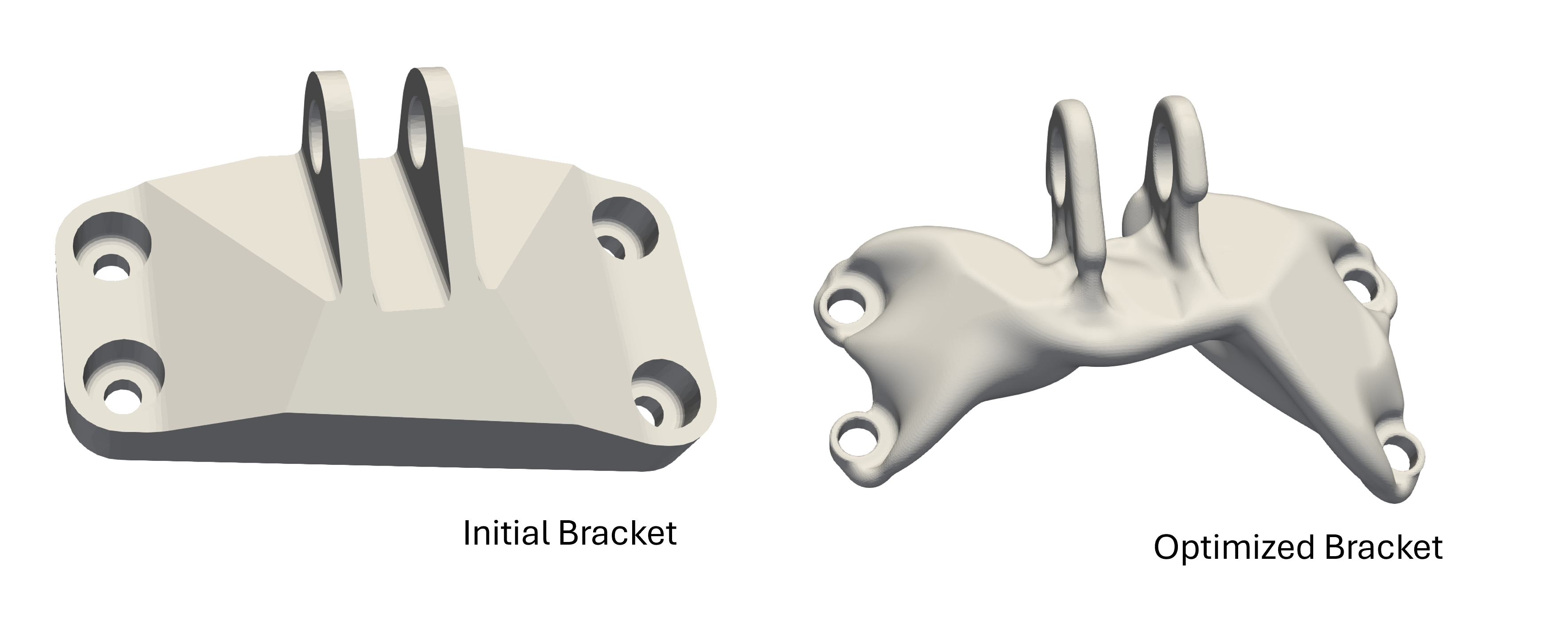
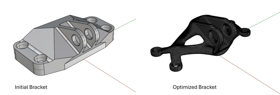
GE Bracket Example
A complete example of performing a LevelOpt bracket optimization
is available along with all geometry files:
bracket geometry,
restraint,
load1,
load2, and a reference
starting design.
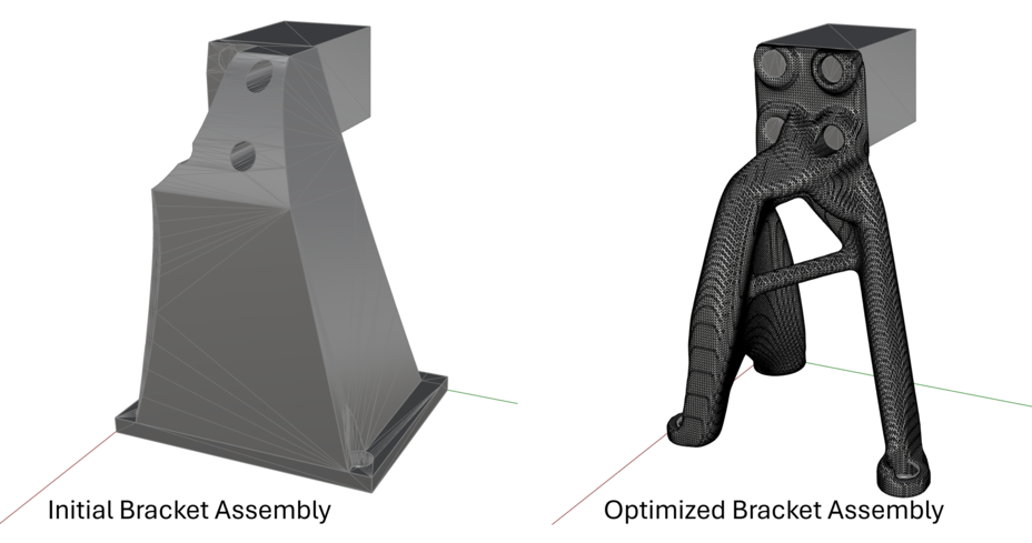
NASA Bracket Assembly Example
A complete example of performing a LevelOpt bracket assembly optimization
is available along with all geometry files:
design geometry,
non-design geometry,
restraint,
load, and a reference
starting design.
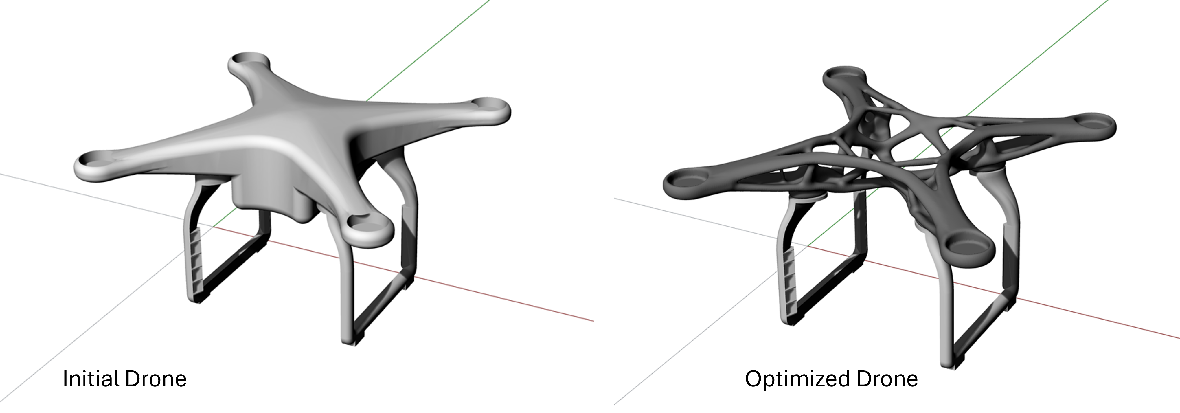
Multiple Load Case Drone Example
A complete example of performing a multi-load LevelOpt drone optimization
is available along with all geometry files:
design geometry,
non-design leg1 geometry,
non-design leg2 geometry,
restraint1,
restraint2,
loads, and a reference
starting design.
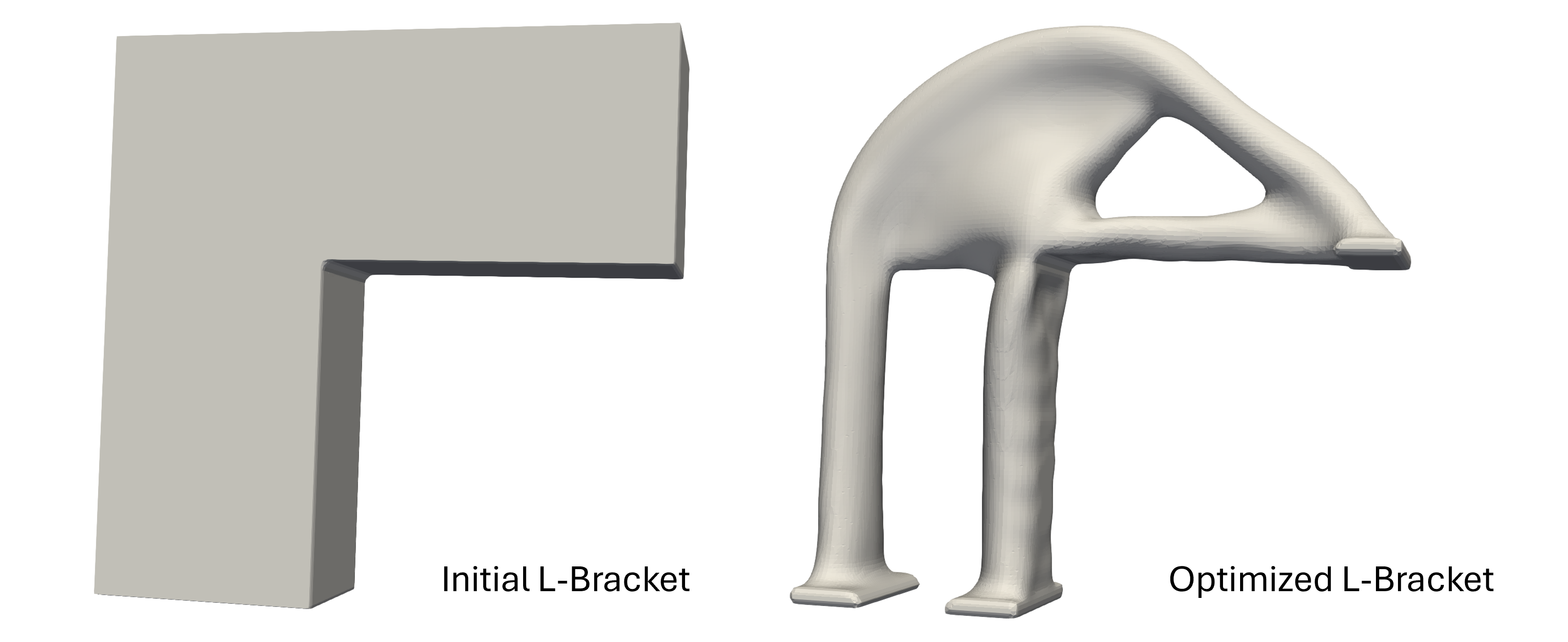
Stress Based L-Bracket Example
A complete example of performing a LevelOpt L-bracket stress-based optimization
is available along with all geometry files:
design geometry,
restraint1,
restraint2,
load, and a reference
final design.
Stress Weighting Example
A complete example of performing a LevelOpt bracket optimization with weighted objectives
is available along with all geometry files: bracket geometry,
restraint,
load1,
load2, and a reference
starting design.